Sageでpandasを使ってみる
manningのMEAP(プレリリース)からデータサイエンティスト育成本(Practical Data Science with R) がでていますが、これをSageを使って試してみようと思い、RのDataFrameのpython版を探していたら、 ggplotで使われているpandasの存在を知りました。
pandasを一言で表現するとRのDataFrameとRDBのSQLを一つにしたような物です。
pandasの基礎
最初に必要なライブラリーをimportします。
|
|
DataFrame
pandasには、たくさんの機能がありますが、DataFrameの基本的な使いかたを簡単にまとめてみます。
DataFrameの作成には、DataFrame関数に列をキーとするマップを引数とします。
   A    B      C
0  4  foo   True
1  3  bar   True
2  1  foo  False
3  2  bar  False
A B C 0 4 foo True 1 3 bar True 2 1 foo False 3 2 bar False |
作成されたDataFrameの情報は、info関数で得ることができます。(もっと詳しい情報は、describe関数を使って得ることができます)
<class 'pandas.core.frame.DataFrame'>
Int64Index: 4 entries, 0 to 3
Data columns (total 3 columns):
A    4 non-null object
B    4 non-null object
C    4 non-null bool
dtypes: bool(1), object(2)
memory usage: 100.0+ bytes
<class 'pandas.core.frame.DataFrame'> Int64Index: 4 entries, 0 to 3 Data columns (total 3 columns): A 4 non-null object B 4 non-null object C 4 non-null bool dtypes: bool(1), object(2) memory usage: 100.0+ bytes |
DataFrameから列を取り出すには、pythonのマップアクセスと同様にキーワード指定(df['B']) で取り出す方法とドット(.)の後にキーワードを付けて指定(df.B)の2つの方法が使えます。 (Rユーザは、変数名をドットで区切ることが多いので注意が必要です)
0    foo
1    bar
2    foo
3    bar
Name: B, dtype: object
0    foo
1    bar
2    foo
3    bar
Name: B, dtype: object
0 foo 1 bar 2 foo 3 bar Name: B, dtype: object 0 foo 1 bar 2 foo 3 bar Name: B, dtype: object |
データフレームの一部を取り出すには、ixを使うのが便利です。 以下の例を出力してみます。
- 0行目を取り出す
- 0行目のA列の要素を取り出す
- 0行から1行のA列からB列(範囲指定では2とCを含まないので注意して下さい)
A       4
B     foo
C    True
Name: 0, dtype: object
4
     B      C
0  foo   True
1  bar   True
2  foo  False
A       4
B     foo
C    True
Name: 0, dtype: object
4
     B      C
0  foo   True
1  bar   True
2  foo  False
|
RのDataFrameと同様に条件に抽出もできます。以下の例では、データフレームdfの列Aの値が1より大きいものを抽出しています。
   A    B      C
0  4  foo   True
1  3  bar   True
3  2  bar  False
A B C 0 4 foo True 1 3 bar True 3 2 bar False |
また列を指定してのソートも簡単です
   A    B      C
2  1  foo  False
3  2  bar  False
1  3  bar   True
0  4  foo   True
A B C 2 1 foo False 3 2 bar False 1 3 bar True 0 4 foo True |
Sageでの出力は、タブ表示の関係で列と値の関係が見にくいので、 html.table関数を使って整形する例を示します。
|
Aggregatin plotting time seriesをsageで試す
DataFrameの基本が何となく分かったところで、ggplotの作者yhat氏の Aggregating & plotting time series in python をSageで試してみます。
使用するデータは、ggplotに付属のアメリカ合衆国の肉のデータ(meat)です。
meatにどのようなデータが入っているのかinfo関数でみてみましょう。日付に続いて肉の種類と出荷量?が入っています。
<class 'pandas.core.frame.DataFrame'>
Int64Index: 827 entries, 0 to 826
Data columns (total 8 columns):
date               827 non-null datetime64[ns]
beef               827 non-null float64
veal               827 non-null float64
pork               827 non-null float64
lamb_and_mutton    827 non-null float64
broilers           635 non-null float64
other_chicken      143 non-null float64
turkey             635 non-null float64
dtypes: datetime64[ns](1), float64(7)
memory usage: 58.1 KB
<class 'pandas.core.frame.DataFrame'> Int64Index: 827 entries, 0 to 826 Data columns (total 8 columns): date 827 non-null datetime64[ns] beef 827 non-null float64 veal 827 non-null float64 pork 827 non-null float64 lamb_and_mutton 827 non-null float64 broilers 635 non-null float64 other_chicken 143 non-null float64 turkey 635 non-null float64 dtypes: datetime64[ns](1), float64(7) memory usage: 58.1 KB |
データの加工
infoの結果、broilers, other_chicken, turkeyは、データ数が827ではないため、存在しないレコード(欠損値)が あることが分かりました。
そこで、欠損値のあるデータから閾値を800として、dropna関数を使ってレコードを抽出します。 (dropnaは欠損値処理の関数なので、その例として使っていると思われます。)
残念ながら、sageにインストールしたpandasでは、axis指定がすべての関数で使えません。そこで転置処理(.T)を使って、 代用しました。
meatは時系列データなので、date列をindexにします。
|
|
データの指定レコードを出力する関数がheadで、終わりはtailです。
           beef veal  pork lamb_and_mutton
date
1944-01-01  751   85  1280              89
1944-02-01  713   77  1169              72
1944-03-01  741   90  1128              75
1944-04-01  650   89   978              66
1944-05-01  681  106  1029              78
1944-06-01  658  125   962              79
1944-07-01  662  142   796              82
1944-08-01  787  175   748              87
1944-09-01  774  182   678              91
1944-10-01  834  215   777             100
beef veal pork lamb_and_mutton date 1944-01-01 751 85 1280 89 1944-02-01 713 77 1169 72 1944-03-01 741 90 1128 75 1944-04-01 650 89 978 66 1944-05-01 681 106 1029 78 1944-06-01 658 125 962 79 1944-07-01 662 142 796 82 1944-08-01 787 175 748 87 1944-09-01 774 182 678 91 1944-10-01 834 215 777 100 |
              beef  veal    pork lamb_and_mutton
date
2012-07-01  2200.8   9.5  1721.8            12.5
2012-08-01  2367.5  10.1  1997.9            14.2
2012-09-01    2016   8.8    1911            12.5
2012-10-01  2343.7  10.3  2210.4            14.2
2012-11-01  2206.6  10.1  2078.7            12.4
beef veal pork lamb_and_mutton date 2012-07-01 2200.8 9.5 1721.8 12.5 2012-08-01 2367.5 10.1 1997.9 14.2 2012-09-01 2016 8.8 1911 12.5 2012-10-01 2343.7 10.3 2210.4 14.2 2012-11-01 2206.6 10.1 2078.7 12.4 |
集計処理
groupbyとsum関数を使うことで、年毎に集計した結果を簡単に計算することができます。
       beef  veal   pork  lamb_and_mutton
1944   8801  1629  11502             1001
1945   9936  1552   8843             1030
1946   9010  1329   9220              946
1947  10096  1493   8811              779
1948   8766  1323   8486              728
1949   9142  1240   8875              587
1950   9248  1137   9397              581
1951   8549   972  10190              508
1952   9337  1080  10321              635
1953  12055  1451   8971              715
beef veal pork lamb_and_mutton 1944 8801 1629 11502 1001 1945 9936 1552 8843 1030 1946 9010 1329 9220 946 1947 10096 1493 8811 779 1948 8766 1323 8486 728 1949 9142 1240 8875 587 1950 9248 1137 9397 581 1951 8549 972 10190 508 1952 9337 1080 10321 635 1953 12055 1451 8971 715 |
また集計された結果もDataFrameなので、ix関数を使って絞り込むことができます。
以下の例では、1940年代のデータのみをthe1940sにセットしています。
|
|
       beef  veal   pork  lamb_and_mutton
1944   8801  1629  11502             1001
1945   9936  1552   8843             1030
1946   9010  1329   9220              946
1947  10096  1493   8811              779
1948   8766  1323   8486              728
1949   9142  1240   8875              587
beef veal pork lamb_and_mutton 1944 8801 1629 11502 1001 1945 9936 1552 8843 1030 1946 9010 1329 9220 946 1947 10096 1493 8811 779 1948 8766 1323 8486 728 1949 9142 1240 8875 587 |
ユーザの定義した関数をgroupbyに指定することができます。
次の例では、floor_decade関数を使ってyearから10年単位に切り捨てた年を計算しています。
|
|
Timestamp('2013-10-09 00:00:00')
Timestamp('2013-10-09 00:00:00')
|
2010 2010 |
floor_decadeを使って簡単に10年毎の集計を求めることができます。
          beef     veal      pork  lamb_and_mutton
1940   55751.0   8566.0   55737.0           5071.0
1950  119161.0  12693.0   98450.0           6724.0
1960  177754.0   8577.0  116587.0           6873.0
1970  228947.0   5713.0  132539.0           4256.0
1980  230100.0   4278.0  150528.0           3394.0
1990  243579.0   2938.0  173519.0           2986.0
2000  260540.7   1685.3  208211.3           1964.7
2010   76391.5    371.9   66491.2            455.6
beef veal pork lamb_and_mutton 1940 55751.0 8566.0 55737.0 5071.0 1950 119161.0 12693.0 98450.0 6724.0 1960 177754.0 8577.0 116587.0 6873.0 1970 228947.0 5713.0 132539.0 4256.0 1980 230100.0 4278.0 150528.0 3394.0 1990 243579.0 2938.0 173519.0 2986.0 2000 260540.7 1685.3 208211.3 1964.7 2010 76391.5 371.9 66491.2 455.6 |
図化
reset_index関数でindexを解除し、値にnameで指定された列名を付けます。
             index  meat sums in the 1940s
0             beef                   55751
1             veal                    8566
2             pork                   55737
3  lamb_and_mutton                    5071
index meat sums in the 1940s 0 beef 55751 1 veal 8566 2 pork 55737 3 lamb_and_mutton 5071 |
by_decadeに10年毎の集計結果を入れ、indexの名前をyearとします。
          beef     veal      pork  lamb_and_mutton
year
1940   55751.0   8566.0   55737.0           5071.0
1950  119161.0  12693.0   98450.0           6724.0
1960  177754.0   8577.0  116587.0           6873.0
1970  228947.0   5713.0  132539.0           4256.0
1980  230100.0   4278.0  150528.0           3394.0
1990  243579.0   2938.0  173519.0           2986.0
2000  260540.7   1685.3  208211.3           1964.7
2010   76391.5    371.9   66491.2            455.6
beef veal pork lamb_and_mutton year 1940 55751.0 8566.0 55737.0 5071.0 1950 119161.0 12693.0 98450.0 6724.0 1960 177754.0 8577.0 116587.0 6873.0 1970 228947.0 5713.0 132539.0 4256.0 1980 230100.0 4278.0 150528.0 3394.0 1990 243579.0 2938.0 173519.0 2986.0 2000 260540.7 1685.3 208211.3 1964.7 2010 76391.5 371.9 66491.2 455.6 |
reset_indexでyearがindexからyear列に変更します。
   year      beef     veal      pork  lamb_and_mutton
0  1940   55751.0   8566.0   55737.0           5071.0
1  1950  119161.0  12693.0   98450.0           6724.0
2  1960  177754.0   8577.0  116587.0           6873.0
3  1970  228947.0   5713.0  132539.0           4256.0
4  1980  230100.0   4278.0  150528.0           3394.0
5  1990  243579.0   2938.0  173519.0           2986.0
6  2000  260540.7   1685.3  208211.3           1964.7
7  2010   76391.5    371.9   66491.2            455.6
year beef veal pork lamb_and_mutton 0 1940 55751.0 8566.0 55737.0 5071.0 1 1950 119161.0 12693.0 98450.0 6724.0 2 1960 177754.0 8577.0 116587.0 6873.0 3 1970 228947.0 5713.0 132539.0 4256.0 4 1980 230100.0 4278.0 150528.0 3394.0 5 1990 243579.0 2938.0 173519.0 2986.0 6 2000 260540.7 1685.3 208211.3 1964.7 7 2010 76391.5 371.9 66491.2 455.6 |
ggplotを使ってby_decadeのbeefの値を棒グラフに表示します。
<ggplot: (8788765854013)> <ggplot: (8788765854013)> |
Saving 11.0 x 8.0 in image. Saving 11.0 x 8.0 in image. 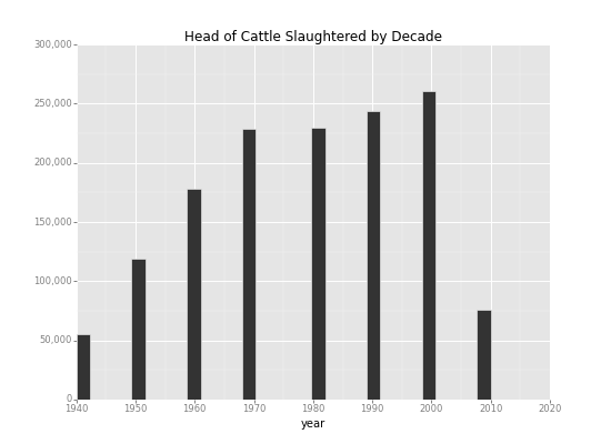
|
melt関数を使ってid_varsでyearをIDとし、列名をvariable列にセットし、値をvalue列にセットした形式に変換します。
   year variable   value
0  1940     beef   55751
1  1950     beef  119161
2  1960     beef  177754
3  1970     beef  228947
4  1980     beef  230100
year variable value 0 1940 beef 55751 1 1950 beef 119161 2 1960 beef 177754 3 1970 beef 228947 4 1980 beef 230100 |
ggplotのaesでweightにvalue, colourにvariableを指定することで、肉の種類別に積み上げられた 棒グラフができました。
<ggplot: (8788768219273)> <ggplot: (8788768219273)> |
Saving 11.0 x 8.0 in image. Saving 11.0 x 8.0 in image. 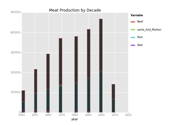
|
時系列の傾向をみる
今度は、meatデータの時系列での傾向をみてみましょう。
meatデータをロードし直し、geom_lineで時系列でプロットします。
<ggplot: (8788765956425)> <ggplot: (8788765956425)> |
Saving 11.0 x 8.0 in image. Saving 11.0 x 8.0 in image. 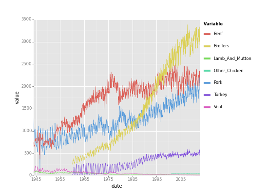
|
stat_smoothのスムージング処理で、時系列データの傾向をプロットしてみます。
<ggplot: (8788765845165)> <ggplot: (8788765845165)> |
Saving 11.0 x 8.0 in image. Saving 11.0 x 8.0 in image. 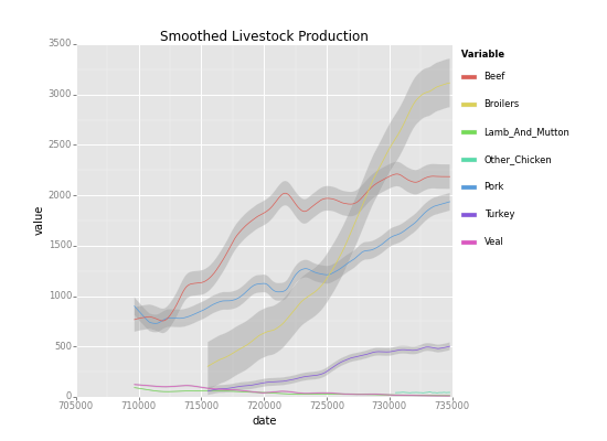
|
|
|